Overview
amRml predicts antimicrobial resistance (AMR) from
bacterial genomic features. It consumes a DuckDB produced by
amRdata and produces ML matrices, tuned logistic regression
models, per-genome predictions, feature importances, and Fisher’s exact
tests as a non-ML baseline.
This vignette uses the Shigella flexneri (Sfl)
DuckDB bundled in inst/extdata.
fixture <- system.file("extdata", "Sfl_parquet.duckdb", package = "amRml")
out_dir <- file.path(tempdir(), "amRml_vignette")
dir.create(out_dir, showWarnings = FALSE, recursive = TRUE)
Generating ML input matrices
generateMLInputs() reads the bug-level DuckDB (metadata
+ feature parquets) and writes one long-format sparse parquet per drug ×
feature × encoding combination into out_path/matrix/. With
stratify_by, it additionally writes year- or
country-stratified matrices into matrix_year/ or
matrix_country/.
generateMLInputs(
  parquet_duckdb_path = fixture,
  out_path            = out_dir,
  n_fold              = 5,
  split               = c(1, 0),
  min_n               = 25,
  verbosity           = "minimal"
)
#> Selected mode: CV (n_fold = 5), train = 1, val = 0, test = 0
#> Matrix output directory: /tmp/Rtmps4Sadm/amRml_vignette/matrix_year
#> Connected to DuckDB for bug: Sfl
#> Building ML matrices for drug_year: FOX_2015-2019
#> Building ML matrices for drug_year: TET_2015-2019
#> Building ML matrices for drug_year: CRO_2015-2019
#> Building ML matrices for drug_year: FEP_2015-2019
#> Building ML matrices for drug_year: TMP_2015-2019
#> Exported matrix: /tmp/Rtmps4Sadm/amRml_vignette/matrix_year/Sfl_drug_year_TMP_2015-2019_genes_counts_sparse.parquet
#> Exported matrix: /tmp/Rtmps4Sadm/amRml_vignette/matrix_year/Sfl_drug_year_TMP_2015-2019_genes_binary_sparse.parquet
#> Exported matrix: /tmp/Rtmps4Sadm/amRml_vignette/matrix_year/Sfl_drug_year_TMP_2015-2019_genes_binary_sparse.parquet
#> Exported matrix: /tmp/Rtmps4Sadm/amRml_vignette/matrix_year/Sfl_drug_year_TMP_2015-2019_proteins_counts_sparse.parquet
#> Exported matrix: /tmp/Rtmps4Sadm/amRml_vignette/matrix_year/Sfl_drug_year_TMP_2015-2019_proteins_binary_sparse.parquet
#> Exported matrix: /tmp/Rtmps4Sadm/amRml_vignette/matrix_year/Sfl_drug_year_TMP_2015-2019_proteins_binary_sparse.parquet
#> Exported matrix: /tmp/Rtmps4Sadm/amRml_vignette/matrix_year/Sfl_drug_year_TMP_2015-2019_domains_counts_sparse.parquet
#> Exported matrix: /tmp/Rtmps4Sadm/amRml_vignette/matrix_year/Sfl_drug_year_TMP_2015-2019_domains_binary_sparse.parquet
#> Exported matrix: /tmp/Rtmps4Sadm/amRml_vignette/matrix_year/Sfl_drug_year_TMP_2015-2019_domains_binary_sparse.parquet
#> Exported matrix: /tmp/Rtmps4Sadm/amRml_vignette/matrix_year/Sfl_drug_year_TMP_2015-2019_struct_binary_sparse.parquet
#> Building ML matrices for drug_year: GEN_2015-2019
#> Building ML matrices for drug_year: AMP_2015-2019
#> Exported matrix: /tmp/Rtmps4Sadm/amRml_vignette/matrix_year/Sfl_drug_year_AMP_2015-2019_genes_counts_sparse.parquet
#> Exported matrix: /tmp/Rtmps4Sadm/amRml_vignette/matrix_year/Sfl_drug_year_AMP_2015-2019_genes_binary_sparse.parquet
#> Exported matrix: /tmp/Rtmps4Sadm/amRml_vignette/matrix_year/Sfl_drug_year_AMP_2015-2019_genes_binary_sparse.parquet
#> Exported matrix: /tmp/Rtmps4Sadm/amRml_vignette/matrix_year/Sfl_drug_year_AMP_2015-2019_proteins_counts_sparse.parquet
#> Exported matrix: /tmp/Rtmps4Sadm/amRml_vignette/matrix_year/Sfl_drug_year_AMP_2015-2019_proteins_binary_sparse.parquet
#> Exported matrix: /tmp/Rtmps4Sadm/amRml_vignette/matrix_year/Sfl_drug_year_AMP_2015-2019_proteins_binary_sparse.parquet
#> Exported matrix: /tmp/Rtmps4Sadm/amRml_vignette/matrix_year/Sfl_drug_year_AMP_2015-2019_domains_counts_sparse.parquet
#> Exported matrix: /tmp/Rtmps4Sadm/amRml_vignette/matrix_year/Sfl_drug_year_AMP_2015-2019_domains_binary_sparse.parquet
#> Exported matrix: /tmp/Rtmps4Sadm/amRml_vignette/matrix_year/Sfl_drug_year_AMP_2015-2019_domains_binary_sparse.parquet
#> Exported matrix: /tmp/Rtmps4Sadm/amRml_vignette/matrix_year/Sfl_drug_year_AMP_2015-2019_struct_binary_sparse.parquet
#> Building ML matrices for drug_year: AMX-CLA_2015-2019
#> Building ML matrices for drug_year: CAZ_2015-2019
#> Building ML matrices for drug_year: SMX_2015-2019
#> Building ML matrices for drug_year: CRO_2010-2014
#> Building ML matrices for drug_year: NAL_2015-2019
#> Building ML matrices for drug_year: CIP_2015-2019
#> Exported matrix: /tmp/Rtmps4Sadm/amRml_vignette/matrix_year/Sfl_drug_year_CIP_2015-2019_genes_counts_sparse.parquet
#> Exported matrix: /tmp/Rtmps4Sadm/amRml_vignette/matrix_year/Sfl_drug_year_CIP_2015-2019_genes_binary_sparse.parquet
#> Exported matrix: /tmp/Rtmps4Sadm/amRml_vignette/matrix_year/Sfl_drug_year_CIP_2015-2019_genes_binary_sparse.parquet
#> Exported matrix: /tmp/Rtmps4Sadm/amRml_vignette/matrix_year/Sfl_drug_year_CIP_2015-2019_proteins_counts_sparse.parquet
#> Exported matrix: /tmp/Rtmps4Sadm/amRml_vignette/matrix_year/Sfl_drug_year_CIP_2015-2019_proteins_binary_sparse.parquet
#> Exported matrix: /tmp/Rtmps4Sadm/amRml_vignette/matrix_year/Sfl_drug_year_CIP_2015-2019_proteins_binary_sparse.parquet
#> Exported matrix: /tmp/Rtmps4Sadm/amRml_vignette/matrix_year/Sfl_drug_year_CIP_2015-2019_domains_counts_sparse.parquet
#> Exported matrix: /tmp/Rtmps4Sadm/amRml_vignette/matrix_year/Sfl_drug_year_CIP_2015-2019_domains_binary_sparse.parquet
#> Exported matrix: /tmp/Rtmps4Sadm/amRml_vignette/matrix_year/Sfl_drug_year_CIP_2015-2019_domains_binary_sparse.parquet
#> Exported matrix: /tmp/Rtmps4Sadm/amRml_vignette/matrix_year/Sfl_drug_year_CIP_2015-2019_struct_binary_sparse.parquet
#> Building ML matrices for drug_year: CTX_2015-2019
#> Building ML matrices for drug_year: CHL_2015-2019
#> Building ML matrices for drug_year: MEM_2015-2019
#> Building ML matrices for drug_year: AZM_2015-2019
#> Exported matrix: /tmp/Rtmps4Sadm/amRml_vignette/matrix_year/Sfl_drug_year_AZM_2015-2019_genes_counts_sparse.parquet
#> Exported matrix: /tmp/Rtmps4Sadm/amRml_vignette/matrix_year/Sfl_drug_year_AZM_2015-2019_genes_binary_sparse.parquet
#> Exported matrix: /tmp/Rtmps4Sadm/amRml_vignette/matrix_year/Sfl_drug_year_AZM_2015-2019_genes_binary_sparse.parquet
#> Exported matrix: /tmp/Rtmps4Sadm/amRml_vignette/matrix_year/Sfl_drug_year_AZM_2015-2019_proteins_counts_sparse.parquet
#> Exported matrix: /tmp/Rtmps4Sadm/amRml_vignette/matrix_year/Sfl_drug_year_AZM_2015-2019_proteins_binary_sparse.parquet
#> Exported matrix: /tmp/Rtmps4Sadm/amRml_vignette/matrix_year/Sfl_drug_year_AZM_2015-2019_proteins_binary_sparse.parquet
#> Exported matrix: /tmp/Rtmps4Sadm/amRml_vignette/matrix_year/Sfl_drug_year_AZM_2015-2019_domains_counts_sparse.parquet
#> Exported matrix: /tmp/Rtmps4Sadm/amRml_vignette/matrix_year/Sfl_drug_year_AZM_2015-2019_domains_binary_sparse.parquet
#> Exported matrix: /tmp/Rtmps4Sadm/amRml_vignette/matrix_year/Sfl_drug_year_AZM_2015-2019_domains_binary_sparse.parquet
#> Exported matrix: /tmp/Rtmps4Sadm/amRml_vignette/matrix_year/Sfl_drug_year_AZM_2015-2019_struct_binary_sparse.parquet
#> Building ML matrices for drug_year: CST_2015-2019
#> Building ML matrices for drug_class_year: CEP_2015-2019
#> Building ML matrices for drug_class_year: AMF_2015-2019
#> Building ML matrices for drug_class_year: POL_2015-2019
#> Building ML matrices for drug_class_year: QUI_2015-2019
#> Building ML matrices for drug_class_year: MAC_2015-2019
#> Exported matrix: /tmp/Rtmps4Sadm/amRml_vignette/matrix_year/Sfl_drug_class_year_MAC_2015-2019_genes_counts_sparse.parquet
#> Exported matrix: /tmp/Rtmps4Sadm/amRml_vignette/matrix_year/Sfl_drug_class_year_MAC_2015-2019_genes_binary_sparse.parquet
#> Exported matrix: /tmp/Rtmps4Sadm/amRml_vignette/matrix_year/Sfl_drug_class_year_MAC_2015-2019_genes_binary_sparse.parquet
#> Exported matrix: /tmp/Rtmps4Sadm/amRml_vignette/matrix_year/Sfl_drug_class_year_MAC_2015-2019_proteins_counts_sparse.parquet
#> Exported matrix: /tmp/Rtmps4Sadm/amRml_vignette/matrix_year/Sfl_drug_class_year_MAC_2015-2019_proteins_binary_sparse.parquet
#> Exported matrix: /tmp/Rtmps4Sadm/amRml_vignette/matrix_year/Sfl_drug_class_year_MAC_2015-2019_proteins_binary_sparse.parquet
#> Exported matrix: /tmp/Rtmps4Sadm/amRml_vignette/matrix_year/Sfl_drug_class_year_MAC_2015-2019_domains_counts_sparse.parquet
#> Exported matrix: /tmp/Rtmps4Sadm/amRml_vignette/matrix_year/Sfl_drug_class_year_MAC_2015-2019_domains_binary_sparse.parquet
#> Exported matrix: /tmp/Rtmps4Sadm/amRml_vignette/matrix_year/Sfl_drug_class_year_MAC_2015-2019_domains_binary_sparse.parquet
#> Exported matrix: /tmp/Rtmps4Sadm/amRml_vignette/matrix_year/Sfl_drug_class_year_MAC_2015-2019_struct_binary_sparse.parquet
#> Building ML matrices for drug_class_year: CEP_2010-2014
#> Building ML matrices for drug_class_year: FLQ_2015-2019
#> Exported matrix: /tmp/Rtmps4Sadm/amRml_vignette/matrix_year/Sfl_drug_class_year_FLQ_2015-2019_genes_counts_sparse.parquet
#> Exported matrix: /tmp/Rtmps4Sadm/amRml_vignette/matrix_year/Sfl_drug_class_year_FLQ_2015-2019_genes_binary_sparse.parquet
#> Exported matrix: /tmp/Rtmps4Sadm/amRml_vignette/matrix_year/Sfl_drug_class_year_FLQ_2015-2019_genes_binary_sparse.parquet
#> Exported matrix: /tmp/Rtmps4Sadm/amRml_vignette/matrix_year/Sfl_drug_class_year_FLQ_2015-2019_proteins_counts_sparse.parquet
#> Exported matrix: /tmp/Rtmps4Sadm/amRml_vignette/matrix_year/Sfl_drug_class_year_FLQ_2015-2019_proteins_binary_sparse.parquet
#> Exported matrix: /tmp/Rtmps4Sadm/amRml_vignette/matrix_year/Sfl_drug_class_year_FLQ_2015-2019_proteins_binary_sparse.parquet
#> Exported matrix: /tmp/Rtmps4Sadm/amRml_vignette/matrix_year/Sfl_drug_class_year_FLQ_2015-2019_domains_counts_sparse.parquet
#> Exported matrix: /tmp/Rtmps4Sadm/amRml_vignette/matrix_year/Sfl_drug_class_year_FLQ_2015-2019_domains_binary_sparse.parquet
#> Exported matrix: /tmp/Rtmps4Sadm/amRml_vignette/matrix_year/Sfl_drug_class_year_FLQ_2015-2019_domains_binary_sparse.parquet
#> Exported matrix: /tmp/Rtmps4Sadm/amRml_vignette/matrix_year/Sfl_drug_class_year_FLQ_2015-2019_struct_binary_sparse.parquet
#> Building ML matrices for drug_class_year: PEN-BLI_2015-2019
#> Building ML matrices for drug_class_year: TET_2015-2019
#> Building ML matrices for drug_class_year: CAR_2015-2019
#> Building ML matrices for drug_class_year: PEN_2015-2019
#> Exported matrix: /tmp/Rtmps4Sadm/amRml_vignette/matrix_year/Sfl_drug_class_year_PEN_2015-2019_genes_counts_sparse.parquet
#> Exported matrix: /tmp/Rtmps4Sadm/amRml_vignette/matrix_year/Sfl_drug_class_year_PEN_2015-2019_genes_binary_sparse.parquet
#> Exported matrix: /tmp/Rtmps4Sadm/amRml_vignette/matrix_year/Sfl_drug_class_year_PEN_2015-2019_genes_binary_sparse.parquet
#> Exported matrix: /tmp/Rtmps4Sadm/amRml_vignette/matrix_year/Sfl_drug_class_year_PEN_2015-2019_proteins_counts_sparse.parquet
#> Exported matrix: /tmp/Rtmps4Sadm/amRml_vignette/matrix_year/Sfl_drug_class_year_PEN_2015-2019_proteins_binary_sparse.parquet
#> Exported matrix: /tmp/Rtmps4Sadm/amRml_vignette/matrix_year/Sfl_drug_class_year_PEN_2015-2019_proteins_binary_sparse.parquet
#> Exported matrix: /tmp/Rtmps4Sadm/amRml_vignette/matrix_year/Sfl_drug_class_year_PEN_2015-2019_domains_counts_sparse.parquet
#> Exported matrix: /tmp/Rtmps4Sadm/amRml_vignette/matrix_year/Sfl_drug_class_year_PEN_2015-2019_domains_binary_sparse.parquet
#> Exported matrix: /tmp/Rtmps4Sadm/amRml_vignette/matrix_year/Sfl_drug_class_year_PEN_2015-2019_domains_binary_sparse.parquet
#> Exported matrix: /tmp/Rtmps4Sadm/amRml_vignette/matrix_year/Sfl_drug_class_year_PEN_2015-2019_struct_binary_sparse.parquet
#> Building ML matrices for drug_class_year: TMD_2015-2019
#> Exported matrix: /tmp/Rtmps4Sadm/amRml_vignette/matrix_year/Sfl_drug_class_year_TMD_2015-2019_genes_counts_sparse.parquet
#> Exported matrix: /tmp/Rtmps4Sadm/amRml_vignette/matrix_year/Sfl_drug_class_year_TMD_2015-2019_genes_binary_sparse.parquet
#> Exported matrix: /tmp/Rtmps4Sadm/amRml_vignette/matrix_year/Sfl_drug_class_year_TMD_2015-2019_genes_binary_sparse.parquet
#> Exported matrix: /tmp/Rtmps4Sadm/amRml_vignette/matrix_year/Sfl_drug_class_year_TMD_2015-2019_proteins_counts_sparse.parquet
#> Exported matrix: /tmp/Rtmps4Sadm/amRml_vignette/matrix_year/Sfl_drug_class_year_TMD_2015-2019_proteins_binary_sparse.parquet
#> Exported matrix: /tmp/Rtmps4Sadm/amRml_vignette/matrix_year/Sfl_drug_class_year_TMD_2015-2019_proteins_binary_sparse.parquet
#> Exported matrix: /tmp/Rtmps4Sadm/amRml_vignette/matrix_year/Sfl_drug_class_year_TMD_2015-2019_domains_counts_sparse.parquet
#> Exported matrix: /tmp/Rtmps4Sadm/amRml_vignette/matrix_year/Sfl_drug_class_year_TMD_2015-2019_domains_binary_sparse.parquet
#> Exported matrix: /tmp/Rtmps4Sadm/amRml_vignette/matrix_year/Sfl_drug_class_year_TMD_2015-2019_domains_binary_sparse.parquet
#> Exported matrix: /tmp/Rtmps4Sadm/amRml_vignette/matrix_year/Sfl_drug_class_year_TMD_2015-2019_struct_binary_sparse.parquet
#> Building ML matrices for drug_class_year: SUL_2015-2019
#> Building ML matrices for drug_class_year: AMG_2015-2019
#> All LOO matrices generated and saved.
#> Matrix output directory: /tmp/Rtmps4Sadm/amRml_vignette/matrix_country
#> Connected to DuckDB for bug: Sfl
#> Building ML matrices for drug_country: FEP_PRT
#> Building ML matrices for drug_country: TMP_PRT
#> Building ML matrices for drug_country: GEN_PRT
#> Building ML matrices for drug_country: AMP_AUS
#> Exported matrix: /tmp/Rtmps4Sadm/amRml_vignette/matrix_country/Sfl_drug_country_AMP_AUS_genes_counts_sparse.parquet
#> Exported matrix: /tmp/Rtmps4Sadm/amRml_vignette/matrix_country/Sfl_drug_country_AMP_AUS_genes_binary_sparse.parquet
#> Exported matrix: /tmp/Rtmps4Sadm/amRml_vignette/matrix_country/Sfl_drug_country_AMP_AUS_genes_binary_sparse.parquet
#> Exported matrix: /tmp/Rtmps4Sadm/amRml_vignette/matrix_country/Sfl_drug_country_AMP_AUS_proteins_counts_sparse.parquet
#> Exported matrix: /tmp/Rtmps4Sadm/amRml_vignette/matrix_country/Sfl_drug_country_AMP_AUS_proteins_binary_sparse.parquet
#> Exported matrix: /tmp/Rtmps4Sadm/amRml_vignette/matrix_country/Sfl_drug_country_AMP_AUS_proteins_binary_sparse.parquet
#> Exported matrix: /tmp/Rtmps4Sadm/amRml_vignette/matrix_country/Sfl_drug_country_AMP_AUS_domains_counts_sparse.parquet
#> Exported matrix: /tmp/Rtmps4Sadm/amRml_vignette/matrix_country/Sfl_drug_country_AMP_AUS_domains_binary_sparse.parquet
#> Exported matrix: /tmp/Rtmps4Sadm/amRml_vignette/matrix_country/Sfl_drug_country_AMP_AUS_domains_binary_sparse.parquet
#> Exported matrix: /tmp/Rtmps4Sadm/amRml_vignette/matrix_country/Sfl_drug_country_AMP_AUS_struct_binary_sparse.parquet
#> Building ML matrices for drug_country: NAL_PRT
#> Building ML matrices for drug_country: CIP_PRT
#> Building ML matrices for drug_country: CTX_PRT
#> Building ML matrices for drug_country: CHL_PRT
#> Building ML matrices for drug_country: MEM_PRT
#> Building ML matrices for drug_country: CRO_AUS
#> Building ML matrices for drug_country: CRO_THA
#> Building ML matrices for drug_country: FOX_PRT
#> Building ML matrices for drug_country: TET_PRT
#> Building ML matrices for drug_country: CIP_AUS
#> Exported matrix: /tmp/Rtmps4Sadm/amRml_vignette/matrix_country/Sfl_drug_country_CIP_AUS_genes_counts_sparse.parquet
#> Exported matrix: /tmp/Rtmps4Sadm/amRml_vignette/matrix_country/Sfl_drug_country_CIP_AUS_genes_binary_sparse.parquet
#> Exported matrix: /tmp/Rtmps4Sadm/amRml_vignette/matrix_country/Sfl_drug_country_CIP_AUS_genes_binary_sparse.parquet
#> Exported matrix: /tmp/Rtmps4Sadm/amRml_vignette/matrix_country/Sfl_drug_country_CIP_AUS_proteins_counts_sparse.parquet
#> Exported matrix: /tmp/Rtmps4Sadm/amRml_vignette/matrix_country/Sfl_drug_country_CIP_AUS_proteins_binary_sparse.parquet
#> Exported matrix: /tmp/Rtmps4Sadm/amRml_vignette/matrix_country/Sfl_drug_country_CIP_AUS_proteins_binary_sparse.parquet
#> Exported matrix: /tmp/Rtmps4Sadm/amRml_vignette/matrix_country/Sfl_drug_country_CIP_AUS_domains_counts_sparse.parquet
#> Exported matrix: /tmp/Rtmps4Sadm/amRml_vignette/matrix_country/Sfl_drug_country_CIP_AUS_domains_binary_sparse.parquet
#> Exported matrix: /tmp/Rtmps4Sadm/amRml_vignette/matrix_country/Sfl_drug_country_CIP_AUS_domains_binary_sparse.parquet
#> Exported matrix: /tmp/Rtmps4Sadm/amRml_vignette/matrix_country/Sfl_drug_country_CIP_AUS_struct_binary_sparse.parquet
#> Building ML matrices for drug_country: MEM_AUS
#> Building ML matrices for drug_country: AZM_AUS
#> Exported matrix: /tmp/Rtmps4Sadm/amRml_vignette/matrix_country/Sfl_drug_country_AZM_AUS_genes_counts_sparse.parquet
#> Exported matrix: /tmp/Rtmps4Sadm/amRml_vignette/matrix_country/Sfl_drug_country_AZM_AUS_genes_binary_sparse.parquet
#> Exported matrix: /tmp/Rtmps4Sadm/amRml_vignette/matrix_country/Sfl_drug_country_AZM_AUS_genes_binary_sparse.parquet
#> Exported matrix: /tmp/Rtmps4Sadm/amRml_vignette/matrix_country/Sfl_drug_country_AZM_AUS_proteins_counts_sparse.parquet
#> Exported matrix: /tmp/Rtmps4Sadm/amRml_vignette/matrix_country/Sfl_drug_country_AZM_AUS_proteins_binary_sparse.parquet
#> Exported matrix: /tmp/Rtmps4Sadm/amRml_vignette/matrix_country/Sfl_drug_country_AZM_AUS_proteins_binary_sparse.parquet
#> Exported matrix: /tmp/Rtmps4Sadm/amRml_vignette/matrix_country/Sfl_drug_country_AZM_AUS_domains_counts_sparse.parquet
#> Exported matrix: /tmp/Rtmps4Sadm/amRml_vignette/matrix_country/Sfl_drug_country_AZM_AUS_domains_binary_sparse.parquet
#> Exported matrix: /tmp/Rtmps4Sadm/amRml_vignette/matrix_country/Sfl_drug_country_AZM_AUS_domains_binary_sparse.parquet
#> Exported matrix: /tmp/Rtmps4Sadm/amRml_vignette/matrix_country/Sfl_drug_country_AZM_AUS_struct_binary_sparse.parquet
#> Building ML matrices for drug_country: CST_THA
#> Building ML matrices for drug_country: AMP_PRT
#> Building ML matrices for drug_country: AMX-CLA_PRT
#> Building ML matrices for drug_country: CAZ_PRT
#> Building ML matrices for drug_country: SMX_PRT
#> Building ML matrices for drug_country: TMP_AUS
#> Exported matrix: /tmp/Rtmps4Sadm/amRml_vignette/matrix_country/Sfl_drug_country_TMP_AUS_genes_counts_sparse.parquet
#> Exported matrix: /tmp/Rtmps4Sadm/amRml_vignette/matrix_country/Sfl_drug_country_TMP_AUS_genes_binary_sparse.parquet
#> Exported matrix: /tmp/Rtmps4Sadm/amRml_vignette/matrix_country/Sfl_drug_country_TMP_AUS_genes_binary_sparse.parquet
#> Exported matrix: /tmp/Rtmps4Sadm/amRml_vignette/matrix_country/Sfl_drug_country_TMP_AUS_proteins_counts_sparse.parquet
#> Exported matrix: /tmp/Rtmps4Sadm/amRml_vignette/matrix_country/Sfl_drug_country_TMP_AUS_proteins_binary_sparse.parquet
#> Exported matrix: /tmp/Rtmps4Sadm/amRml_vignette/matrix_country/Sfl_drug_country_TMP_AUS_proteins_binary_sparse.parquet
#> Exported matrix: /tmp/Rtmps4Sadm/amRml_vignette/matrix_country/Sfl_drug_country_TMP_AUS_domains_counts_sparse.parquet
#> Exported matrix: /tmp/Rtmps4Sadm/amRml_vignette/matrix_country/Sfl_drug_country_TMP_AUS_domains_binary_sparse.parquet
#> Exported matrix: /tmp/Rtmps4Sadm/amRml_vignette/matrix_country/Sfl_drug_country_TMP_AUS_domains_binary_sparse.parquet
#> Exported matrix: /tmp/Rtmps4Sadm/amRml_vignette/matrix_country/Sfl_drug_country_TMP_AUS_struct_binary_sparse.parquet
#> Building ML matrices for drug_country: GEN_AUS
#> Building ML matrices for drug_class_country: QUI_PRT
#> Building ML matrices for drug_class_country: FLQ_AUS
#> Exported matrix: /tmp/Rtmps4Sadm/amRml_vignette/matrix_country/Sfl_drug_class_country_FLQ_AUS_genes_counts_sparse.parquet
#> Exported matrix: /tmp/Rtmps4Sadm/amRml_vignette/matrix_country/Sfl_drug_class_country_FLQ_AUS_genes_binary_sparse.parquet
#> Exported matrix: /tmp/Rtmps4Sadm/amRml_vignette/matrix_country/Sfl_drug_class_country_FLQ_AUS_genes_binary_sparse.parquet
#> Exported matrix: /tmp/Rtmps4Sadm/amRml_vignette/matrix_country/Sfl_drug_class_country_FLQ_AUS_proteins_counts_sparse.parquet
#> Exported matrix: /tmp/Rtmps4Sadm/amRml_vignette/matrix_country/Sfl_drug_class_country_FLQ_AUS_proteins_binary_sparse.parquet
#> Exported matrix: /tmp/Rtmps4Sadm/amRml_vignette/matrix_country/Sfl_drug_class_country_FLQ_AUS_proteins_binary_sparse.parquet
#> Exported matrix: /tmp/Rtmps4Sadm/amRml_vignette/matrix_country/Sfl_drug_class_country_FLQ_AUS_domains_counts_sparse.parquet
#> Exported matrix: /tmp/Rtmps4Sadm/amRml_vignette/matrix_country/Sfl_drug_class_country_FLQ_AUS_domains_binary_sparse.parquet
#> Exported matrix: /tmp/Rtmps4Sadm/amRml_vignette/matrix_country/Sfl_drug_class_country_FLQ_AUS_domains_binary_sparse.parquet
#> Exported matrix: /tmp/Rtmps4Sadm/amRml_vignette/matrix_country/Sfl_drug_class_country_FLQ_AUS_struct_binary_sparse.parquet
#> Building ML matrices for drug_class_country: CAR_AUS
#> Building ML matrices for drug_class_country: CEP_PRT
#> Building ML matrices for drug_class_country: AMF_PRT
#> Building ML matrices for drug_class_country: PEN_AUS
#> Exported matrix: /tmp/Rtmps4Sadm/amRml_vignette/matrix_country/Sfl_drug_class_country_PEN_AUS_genes_counts_sparse.parquet
#> Exported matrix: /tmp/Rtmps4Sadm/amRml_vignette/matrix_country/Sfl_drug_class_country_PEN_AUS_genes_binary_sparse.parquet
#> Exported matrix: /tmp/Rtmps4Sadm/amRml_vignette/matrix_country/Sfl_drug_class_country_PEN_AUS_genes_binary_sparse.parquet
#> Exported matrix: /tmp/Rtmps4Sadm/amRml_vignette/matrix_country/Sfl_drug_class_country_PEN_AUS_proteins_counts_sparse.parquet
#> Exported matrix: /tmp/Rtmps4Sadm/amRml_vignette/matrix_country/Sfl_drug_class_country_PEN_AUS_proteins_binary_sparse.parquet
#> Exported matrix: /tmp/Rtmps4Sadm/amRml_vignette/matrix_country/Sfl_drug_class_country_PEN_AUS_proteins_binary_sparse.parquet
#> Exported matrix: /tmp/Rtmps4Sadm/amRml_vignette/matrix_country/Sfl_drug_class_country_PEN_AUS_domains_counts_sparse.parquet
#> Exported matrix: /tmp/Rtmps4Sadm/amRml_vignette/matrix_country/Sfl_drug_class_country_PEN_AUS_domains_binary_sparse.parquet
#> Exported matrix: /tmp/Rtmps4Sadm/amRml_vignette/matrix_country/Sfl_drug_class_country_PEN_AUS_domains_binary_sparse.parquet
#> Exported matrix: /tmp/Rtmps4Sadm/amRml_vignette/matrix_country/Sfl_drug_class_country_PEN_AUS_struct_binary_sparse.parquet
#> Building ML matrices for drug_class_country: TMD_AUS
#> Exported matrix: /tmp/Rtmps4Sadm/amRml_vignette/matrix_country/Sfl_drug_class_country_TMD_AUS_genes_counts_sparse.parquet
#> Exported matrix: /tmp/Rtmps4Sadm/amRml_vignette/matrix_country/Sfl_drug_class_country_TMD_AUS_genes_binary_sparse.parquet
#> Exported matrix: /tmp/Rtmps4Sadm/amRml_vignette/matrix_country/Sfl_drug_class_country_TMD_AUS_genes_binary_sparse.parquet
#> Exported matrix: /tmp/Rtmps4Sadm/amRml_vignette/matrix_country/Sfl_drug_class_country_TMD_AUS_proteins_counts_sparse.parquet
#> Exported matrix: /tmp/Rtmps4Sadm/amRml_vignette/matrix_country/Sfl_drug_class_country_TMD_AUS_proteins_binary_sparse.parquet
#> Exported matrix: /tmp/Rtmps4Sadm/amRml_vignette/matrix_country/Sfl_drug_class_country_TMD_AUS_proteins_binary_sparse.parquet
#> Exported matrix: /tmp/Rtmps4Sadm/amRml_vignette/matrix_country/Sfl_drug_class_country_TMD_AUS_domains_counts_sparse.parquet
#> Exported matrix: /tmp/Rtmps4Sadm/amRml_vignette/matrix_country/Sfl_drug_class_country_TMD_AUS_domains_binary_sparse.parquet
#> Exported matrix: /tmp/Rtmps4Sadm/amRml_vignette/matrix_country/Sfl_drug_class_country_TMD_AUS_domains_binary_sparse.parquet
#> Exported matrix: /tmp/Rtmps4Sadm/amRml_vignette/matrix_country/Sfl_drug_class_country_TMD_AUS_struct_binary_sparse.parquet
#> Building ML matrices for drug_class_country: AMG_AUS
#> Building ML matrices for drug_class_country: PEN_PRT
#> Building ML matrices for drug_class_country: TMD_PRT
#> Building ML matrices for drug_class_country: SUL_PRT
#> Building ML matrices for drug_class_country: AMG_PRT
#> Building ML matrices for drug_class_country: CEP_AUS
#> Building ML matrices for drug_class_country: POL_THA
#> Building ML matrices for drug_class_country: CEP_THA
#> Building ML matrices for drug_class_country: FLQ_PRT
#> Building ML matrices for drug_class_country: PEN-BLI_PRT
#> Building ML matrices for drug_class_country: TET_PRT
#> Building ML matrices for drug_class_country: CAR_PRT
#> Building ML matrices for drug_class_country: MAC_AUS
#> Exported matrix: /tmp/Rtmps4Sadm/amRml_vignette/matrix_country/Sfl_drug_class_country_MAC_AUS_genes_counts_sparse.parquet
#> Exported matrix: /tmp/Rtmps4Sadm/amRml_vignette/matrix_country/Sfl_drug_class_country_MAC_AUS_genes_binary_sparse.parquet
#> Exported matrix: /tmp/Rtmps4Sadm/amRml_vignette/matrix_country/Sfl_drug_class_country_MAC_AUS_genes_binary_sparse.parquet
#> Exported matrix: /tmp/Rtmps4Sadm/amRml_vignette/matrix_country/Sfl_drug_class_country_MAC_AUS_proteins_counts_sparse.parquet
#> Exported matrix: /tmp/Rtmps4Sadm/amRml_vignette/matrix_country/Sfl_drug_class_country_MAC_AUS_proteins_binary_sparse.parquet
#> Exported matrix: /tmp/Rtmps4Sadm/amRml_vignette/matrix_country/Sfl_drug_class_country_MAC_AUS_proteins_binary_sparse.parquet
#> Exported matrix: /tmp/Rtmps4Sadm/amRml_vignette/matrix_country/Sfl_drug_class_country_MAC_AUS_domains_counts_sparse.parquet
#> Exported matrix: /tmp/Rtmps4Sadm/amRml_vignette/matrix_country/Sfl_drug_class_country_MAC_AUS_domains_binary_sparse.parquet
#> Exported matrix: /tmp/Rtmps4Sadm/amRml_vignette/matrix_country/Sfl_drug_class_country_MAC_AUS_domains_binary_sparse.parquet
#> Exported matrix: /tmp/Rtmps4Sadm/amRml_vignette/matrix_country/Sfl_drug_class_country_MAC_AUS_struct_binary_sparse.parquet
#> All LOO matrices generated and saved.
#> Matrix output directory: /tmp/Rtmps4Sadm/amRml_vignette/matrix
#> Connected to DuckDB for bug: Sfl
#> Building ML matrices for drug: AMP
#> Exported matrix: /tmp/Rtmps4Sadm/amRml_vignette/matrix/Sfl_drug_AMP_genes_counts_sparse.parquet
#> Exported matrix: /tmp/Rtmps4Sadm/amRml_vignette/matrix/Sfl_drug_AMP_genes_binary_sparse.parquet
#> Exported matrix: /tmp/Rtmps4Sadm/amRml_vignette/matrix/Sfl_drug_AMP_genes_binary_sparse.parquet
#> Exported matrix: /tmp/Rtmps4Sadm/amRml_vignette/matrix/Sfl_drug_AMP_proteins_counts_sparse.parquet
#> Exported matrix: /tmp/Rtmps4Sadm/amRml_vignette/matrix/Sfl_drug_AMP_proteins_binary_sparse.parquet
#> Exported matrix: /tmp/Rtmps4Sadm/amRml_vignette/matrix/Sfl_drug_AMP_proteins_binary_sparse.parquet
#> Exported matrix: /tmp/Rtmps4Sadm/amRml_vignette/matrix/Sfl_drug_AMP_domains_counts_sparse.parquet
#> Exported matrix: /tmp/Rtmps4Sadm/amRml_vignette/matrix/Sfl_drug_AMP_domains_binary_sparse.parquet
#> Exported matrix: /tmp/Rtmps4Sadm/amRml_vignette/matrix/Sfl_drug_AMP_domains_binary_sparse.parquet
#> Exported matrix: /tmp/Rtmps4Sadm/amRml_vignette/matrix/Sfl_drug_AMP_struct_binary_sparse.parquet
#> Building ML matrices for drug: AMX-CLA
#> Building ML matrices for drug: TMP
#> Exported matrix: /tmp/Rtmps4Sadm/amRml_vignette/matrix/Sfl_drug_TMP_genes_counts_sparse.parquet
#> Exported matrix: /tmp/Rtmps4Sadm/amRml_vignette/matrix/Sfl_drug_TMP_genes_binary_sparse.parquet
#> Exported matrix: /tmp/Rtmps4Sadm/amRml_vignette/matrix/Sfl_drug_TMP_genes_binary_sparse.parquet
#> Exported matrix: /tmp/Rtmps4Sadm/amRml_vignette/matrix/Sfl_drug_TMP_proteins_counts_sparse.parquet
#> Exported matrix: /tmp/Rtmps4Sadm/amRml_vignette/matrix/Sfl_drug_TMP_proteins_binary_sparse.parquet
#> Exported matrix: /tmp/Rtmps4Sadm/amRml_vignette/matrix/Sfl_drug_TMP_proteins_binary_sparse.parquet
#> Exported matrix: /tmp/Rtmps4Sadm/amRml_vignette/matrix/Sfl_drug_TMP_domains_counts_sparse.parquet
#> Exported matrix: /tmp/Rtmps4Sadm/amRml_vignette/matrix/Sfl_drug_TMP_domains_binary_sparse.parquet
#> Exported matrix: /tmp/Rtmps4Sadm/amRml_vignette/matrix/Sfl_drug_TMP_domains_binary_sparse.parquet
#> Exported matrix: /tmp/Rtmps4Sadm/amRml_vignette/matrix/Sfl_drug_TMP_struct_binary_sparse.parquet
#> Building ML matrices for drug: SXZ
#> Building ML matrices for drug: AZM
#> Exported matrix: /tmp/Rtmps4Sadm/amRml_vignette/matrix/Sfl_drug_AZM_genes_counts_sparse.parquet
#> Exported matrix: /tmp/Rtmps4Sadm/amRml_vignette/matrix/Sfl_drug_AZM_genes_binary_sparse.parquet
#> Exported matrix: /tmp/Rtmps4Sadm/amRml_vignette/matrix/Sfl_drug_AZM_genes_binary_sparse.parquet
#> Exported matrix: /tmp/Rtmps4Sadm/amRml_vignette/matrix/Sfl_drug_AZM_proteins_counts_sparse.parquet
#> Exported matrix: /tmp/Rtmps4Sadm/amRml_vignette/matrix/Sfl_drug_AZM_proteins_binary_sparse.parquet
#> Exported matrix: /tmp/Rtmps4Sadm/amRml_vignette/matrix/Sfl_drug_AZM_proteins_binary_sparse.parquet
#> Exported matrix: /tmp/Rtmps4Sadm/amRml_vignette/matrix/Sfl_drug_AZM_domains_counts_sparse.parquet
#> Exported matrix: /tmp/Rtmps4Sadm/amRml_vignette/matrix/Sfl_drug_AZM_domains_binary_sparse.parquet
#> Exported matrix: /tmp/Rtmps4Sadm/amRml_vignette/matrix/Sfl_drug_AZM_domains_binary_sparse.parquet
#> Exported matrix: /tmp/Rtmps4Sadm/amRml_vignette/matrix/Sfl_drug_AZM_struct_binary_sparse.parquet
#> Building ML matrices for drug: CTX
#> Building ML matrices for drug: FOX
#> Building ML matrices for drug: FEP
#> Building ML matrices for drug: SMX
#> Building ML matrices for drug: MEM
#> Building ML matrices for drug: CAZ
#> Building ML matrices for drug: TET
#> Building ML matrices for drug: CHL
#> Building ML matrices for drug: TMP-SMX
#> Building ML matrices for drug: CST
#> Building ML matrices for drug: NAL
#> Building ML matrices for drug: CIP
#> Exported matrix: /tmp/Rtmps4Sadm/amRml_vignette/matrix/Sfl_drug_CIP_genes_counts_sparse.parquet
#> Exported matrix: /tmp/Rtmps4Sadm/amRml_vignette/matrix/Sfl_drug_CIP_genes_binary_sparse.parquet
#> Exported matrix: /tmp/Rtmps4Sadm/amRml_vignette/matrix/Sfl_drug_CIP_genes_binary_sparse.parquet
#> Exported matrix: /tmp/Rtmps4Sadm/amRml_vignette/matrix/Sfl_drug_CIP_proteins_counts_sparse.parquet
#> Exported matrix: /tmp/Rtmps4Sadm/amRml_vignette/matrix/Sfl_drug_CIP_proteins_binary_sparse.parquet
#> Exported matrix: /tmp/Rtmps4Sadm/amRml_vignette/matrix/Sfl_drug_CIP_proteins_binary_sparse.parquet
#> Exported matrix: /tmp/Rtmps4Sadm/amRml_vignette/matrix/Sfl_drug_CIP_domains_counts_sparse.parquet
#> Exported matrix: /tmp/Rtmps4Sadm/amRml_vignette/matrix/Sfl_drug_CIP_domains_binary_sparse.parquet
#> Exported matrix: /tmp/Rtmps4Sadm/amRml_vignette/matrix/Sfl_drug_CIP_domains_binary_sparse.parquet
#> Exported matrix: /tmp/Rtmps4Sadm/amRml_vignette/matrix/Sfl_drug_CIP_struct_binary_sparse.parquet
#> Building ML matrices for drug: GEN
#> Building ML matrices for drug: CRO
#> Exported matrix: /tmp/Rtmps4Sadm/amRml_vignette/matrix/Sfl_drug_CRO_genes_counts_sparse.parquet
#> Exported matrix: /tmp/Rtmps4Sadm/amRml_vignette/matrix/Sfl_drug_CRO_genes_binary_sparse.parquet
#> Exported matrix: /tmp/Rtmps4Sadm/amRml_vignette/matrix/Sfl_drug_CRO_genes_binary_sparse.parquet
#> Exported matrix: /tmp/Rtmps4Sadm/amRml_vignette/matrix/Sfl_drug_CRO_proteins_counts_sparse.parquet
#> Exported matrix: /tmp/Rtmps4Sadm/amRml_vignette/matrix/Sfl_drug_CRO_proteins_binary_sparse.parquet
#> Exported matrix: /tmp/Rtmps4Sadm/amRml_vignette/matrix/Sfl_drug_CRO_proteins_binary_sparse.parquet
#> Exported matrix: /tmp/Rtmps4Sadm/amRml_vignette/matrix/Sfl_drug_CRO_domains_counts_sparse.parquet
#> Exported matrix: /tmp/Rtmps4Sadm/amRml_vignette/matrix/Sfl_drug_CRO_domains_binary_sparse.parquet
#> Exported matrix: /tmp/Rtmps4Sadm/amRml_vignette/matrix/Sfl_drug_CRO_domains_binary_sparse.parquet
#> Exported matrix: /tmp/Rtmps4Sadm/amRml_vignette/matrix/Sfl_drug_CRO_struct_binary_sparse.parquet
#> Building ML matrices for drug_class: SUL
#> Building ML matrices for drug_class: TMD-SUL
#> Building ML matrices for drug_class: MAC
#> Exported matrix: /tmp/Rtmps4Sadm/amRml_vignette/matrix/Sfl_drug_class_MAC_genes_counts_sparse.parquet
#> Exported matrix: /tmp/Rtmps4Sadm/amRml_vignette/matrix/Sfl_drug_class_MAC_genes_binary_sparse.parquet
#> Exported matrix: /tmp/Rtmps4Sadm/amRml_vignette/matrix/Sfl_drug_class_MAC_genes_binary_sparse.parquet
#> Exported matrix: /tmp/Rtmps4Sadm/amRml_vignette/matrix/Sfl_drug_class_MAC_proteins_counts_sparse.parquet
#> Exported matrix: /tmp/Rtmps4Sadm/amRml_vignette/matrix/Sfl_drug_class_MAC_proteins_binary_sparse.parquet
#> Exported matrix: /tmp/Rtmps4Sadm/amRml_vignette/matrix/Sfl_drug_class_MAC_proteins_binary_sparse.parquet
#> Exported matrix: /tmp/Rtmps4Sadm/amRml_vignette/matrix/Sfl_drug_class_MAC_domains_counts_sparse.parquet
#> Exported matrix: /tmp/Rtmps4Sadm/amRml_vignette/matrix/Sfl_drug_class_MAC_domains_binary_sparse.parquet
#> Exported matrix: /tmp/Rtmps4Sadm/amRml_vignette/matrix/Sfl_drug_class_MAC_domains_binary_sparse.parquet
#> Exported matrix: /tmp/Rtmps4Sadm/amRml_vignette/matrix/Sfl_drug_class_MAC_struct_binary_sparse.parquet
#> Building ML matrices for drug_class: POL
#> Building ML matrices for drug_class: AMF
#> Building ML matrices for drug_class: QUI
#> Building ML matrices for drug_class: FLQ
#> Exported matrix: /tmp/Rtmps4Sadm/amRml_vignette/matrix/Sfl_drug_class_FLQ_genes_counts_sparse.parquet
#> Exported matrix: /tmp/Rtmps4Sadm/amRml_vignette/matrix/Sfl_drug_class_FLQ_genes_binary_sparse.parquet
#> Exported matrix: /tmp/Rtmps4Sadm/amRml_vignette/matrix/Sfl_drug_class_FLQ_genes_binary_sparse.parquet
#> Exported matrix: /tmp/Rtmps4Sadm/amRml_vignette/matrix/Sfl_drug_class_FLQ_proteins_counts_sparse.parquet
#> Exported matrix: /tmp/Rtmps4Sadm/amRml_vignette/matrix/Sfl_drug_class_FLQ_proteins_binary_sparse.parquet
#> Exported matrix: /tmp/Rtmps4Sadm/amRml_vignette/matrix/Sfl_drug_class_FLQ_proteins_binary_sparse.parquet
#> Exported matrix: /tmp/Rtmps4Sadm/amRml_vignette/matrix/Sfl_drug_class_FLQ_domains_counts_sparse.parquet
#> Exported matrix: /tmp/Rtmps4Sadm/amRml_vignette/matrix/Sfl_drug_class_FLQ_domains_binary_sparse.parquet
#> Exported matrix: /tmp/Rtmps4Sadm/amRml_vignette/matrix/Sfl_drug_class_FLQ_domains_binary_sparse.parquet
#> Exported matrix: /tmp/Rtmps4Sadm/amRml_vignette/matrix/Sfl_drug_class_FLQ_struct_binary_sparse.parquet
#> Building ML matrices for drug_class: PEN
#> Exported matrix: /tmp/Rtmps4Sadm/amRml_vignette/matrix/Sfl_drug_class_PEN_genes_counts_sparse.parquet
#> Exported matrix: /tmp/Rtmps4Sadm/amRml_vignette/matrix/Sfl_drug_class_PEN_genes_binary_sparse.parquet
#> Exported matrix: /tmp/Rtmps4Sadm/amRml_vignette/matrix/Sfl_drug_class_PEN_genes_binary_sparse.parquet
#> Exported matrix: /tmp/Rtmps4Sadm/amRml_vignette/matrix/Sfl_drug_class_PEN_proteins_counts_sparse.parquet
#> Exported matrix: /tmp/Rtmps4Sadm/amRml_vignette/matrix/Sfl_drug_class_PEN_proteins_binary_sparse.parquet
#> Exported matrix: /tmp/Rtmps4Sadm/amRml_vignette/matrix/Sfl_drug_class_PEN_proteins_binary_sparse.parquet
#> Exported matrix: /tmp/Rtmps4Sadm/amRml_vignette/matrix/Sfl_drug_class_PEN_domains_counts_sparse.parquet
#> Exported matrix: /tmp/Rtmps4Sadm/amRml_vignette/matrix/Sfl_drug_class_PEN_domains_binary_sparse.parquet
#> Exported matrix: /tmp/Rtmps4Sadm/amRml_vignette/matrix/Sfl_drug_class_PEN_domains_binary_sparse.parquet
#> Exported matrix: /tmp/Rtmps4Sadm/amRml_vignette/matrix/Sfl_drug_class_PEN_struct_binary_sparse.parquet
#> Building ML matrices for drug_class: PEN-BLI
#> Building ML matrices for drug_class: CEP
#> Exported matrix: /tmp/Rtmps4Sadm/amRml_vignette/matrix/Sfl_drug_class_CEP_genes_counts_sparse.parquet
#> Exported matrix: /tmp/Rtmps4Sadm/amRml_vignette/matrix/Sfl_drug_class_CEP_genes_binary_sparse.parquet
#> Exported matrix: /tmp/Rtmps4Sadm/amRml_vignette/matrix/Sfl_drug_class_CEP_genes_binary_sparse.parquet
#> Exported matrix: /tmp/Rtmps4Sadm/amRml_vignette/matrix/Sfl_drug_class_CEP_proteins_counts_sparse.parquet
#> Exported matrix: /tmp/Rtmps4Sadm/amRml_vignette/matrix/Sfl_drug_class_CEP_proteins_binary_sparse.parquet
#> Exported matrix: /tmp/Rtmps4Sadm/amRml_vignette/matrix/Sfl_drug_class_CEP_proteins_binary_sparse.parquet
#> Exported matrix: /tmp/Rtmps4Sadm/amRml_vignette/matrix/Sfl_drug_class_CEP_domains_counts_sparse.parquet
#> Exported matrix: /tmp/Rtmps4Sadm/amRml_vignette/matrix/Sfl_drug_class_CEP_domains_binary_sparse.parquet
#> Exported matrix: /tmp/Rtmps4Sadm/amRml_vignette/matrix/Sfl_drug_class_CEP_domains_binary_sparse.parquet
#> Exported matrix: /tmp/Rtmps4Sadm/amRml_vignette/matrix/Sfl_drug_class_CEP_struct_binary_sparse.parquet
#> Building ML matrices for drug_class: TET
#> Building ML matrices for drug_class: TMD
#> Exported matrix: /tmp/Rtmps4Sadm/amRml_vignette/matrix/Sfl_drug_class_TMD_genes_counts_sparse.parquet
#> Exported matrix: /tmp/Rtmps4Sadm/amRml_vignette/matrix/Sfl_drug_class_TMD_genes_binary_sparse.parquet
#> Exported matrix: /tmp/Rtmps4Sadm/amRml_vignette/matrix/Sfl_drug_class_TMD_genes_binary_sparse.parquet
#> Exported matrix: /tmp/Rtmps4Sadm/amRml_vignette/matrix/Sfl_drug_class_TMD_proteins_counts_sparse.parquet
#> Exported matrix: /tmp/Rtmps4Sadm/amRml_vignette/matrix/Sfl_drug_class_TMD_proteins_binary_sparse.parquet
#> Exported matrix: /tmp/Rtmps4Sadm/amRml_vignette/matrix/Sfl_drug_class_TMD_proteins_binary_sparse.parquet
#> Exported matrix: /tmp/Rtmps4Sadm/amRml_vignette/matrix/Sfl_drug_class_TMD_domains_counts_sparse.parquet
#> Exported matrix: /tmp/Rtmps4Sadm/amRml_vignette/matrix/Sfl_drug_class_TMD_domains_binary_sparse.parquet
#> Exported matrix: /tmp/Rtmps4Sadm/amRml_vignette/matrix/Sfl_drug_class_TMD_domains_binary_sparse.parquet
#> Exported matrix: /tmp/Rtmps4Sadm/amRml_vignette/matrix/Sfl_drug_class_TMD_struct_binary_sparse.parquet
#> Building ML matrices for drug_class: AMG
#> Building ML matrices for drug_class: CAR
#> Building MDR matrices for classes: PEN, PEN_TMD, TMD_MAC_PEN, TMD_PEN, TMD_PEN_MAC
#> Exported MDR matrix: /tmp/Rtmps4Sadm/amRml_vignette/MDR_matrix/Sfl_MDR_resistant_classes_genes_counts_sparse.parquet
#> Exported MDR matrix: /tmp/Rtmps4Sadm/amRml_vignette/MDR_matrix/Sfl_MDR_resistant_classes_genes_binary_sparse.parquet
#> Exported MDR matrix: /tmp/Rtmps4Sadm/amRml_vignette/MDR_matrix/Sfl_MDR_resistant_classes_genes_binary_sparse.parquet
#> Exported MDR matrix: /tmp/Rtmps4Sadm/amRml_vignette/MDR_matrix/Sfl_MDR_resistant_classes_proteins_counts_sparse.parquet
#> Exported MDR matrix: /tmp/Rtmps4Sadm/amRml_vignette/MDR_matrix/Sfl_MDR_resistant_classes_proteins_binary_sparse.parquet
#> Exported MDR matrix: /tmp/Rtmps4Sadm/amRml_vignette/MDR_matrix/Sfl_MDR_resistant_classes_proteins_binary_sparse.parquet
#> Exported MDR matrix: /tmp/Rtmps4Sadm/amRml_vignette/MDR_matrix/Sfl_MDR_resistant_classes_domains_counts_sparse.parquet
#> Exported MDR matrix: /tmp/Rtmps4Sadm/amRml_vignette/MDR_matrix/Sfl_MDR_resistant_classes_domains_binary_sparse.parquet
#> Exported MDR matrix: /tmp/Rtmps4Sadm/amRml_vignette/MDR_matrix/Sfl_MDR_resistant_classes_domains_binary_sparse.parquet
#> Exported MDR matrix: /tmp/Rtmps4Sadm/amRml_vignette/MDR_matrix/Sfl_MDR_resistant_classes_struct_binary_sparse.parquet
#> The MDR matrix has been generated and saved.
#> All cross-drug testing matrices generated
#> All LOO-drug matrices generated with genome-level blocking
#> All matrices generated and saved.

list.files(file.path(out_dir, "matrix"))[1:5]
#> [1] "Sfl_drug_AMP_domains_binary_sparse.parquet"
#> [2] "Sfl_drug_AMP_domains_counts_sparse.parquet"
#> [3] "Sfl_drug_AMP_genes_binary_sparse.parquet"
#> [4] "Sfl_drug_AMP_genes_counts_sparse.parquet"
#> [5] "Sfl_drug_AMP_proteins_binary_sparse.parquet"
For a classical train/validation/test split instead of
cross-validation, set n_fold = NULL and pass a length-2
split of c(train_prop, val_prop); the test
proportion is the remainder.
generateMLInputs(
  parquet_duckdb_path = fixture,
  out_path            = out_dir,
  n_fold              = NULL,
  split               = c(0.7, 0.15),
  verbosity           = "debug"
)
Loading a single matrix
The generated parquets are long-format sparse tibbles with these columns:
| Column | Description |
|---|---|
genome_id |
Unique identifier for each isolate |
feature_id |
Feature name (gene, protein, domain, or struct) |
value |
Binary presence/absence (0/1) or count |
genome_drug.resistant_phenotype |
"Resistant" or "Susceptible"
|
loadMLInputTibble() converts one of them to wide format
(one row per genome, one column per feature) ready for ML.
matrix_path <- file.path(
  out_dir, "matrix", "Sfl_drug_AMP_genes_binary_sparse.parquet"
)

ml_tibble <- loadMLInputTibble(matrix_path)
n_features <- getNumFeat(ml_tibble)
target_var <- .getTargetVarName(ml_tibble)

c(n_features = n_features, target_var = target_var)
#> $n_features
#> [1] 6946
#>
#> $target_var
#> genome_drug.resistant_phenotype
Per-matrix pipeline
runMLPipeline() runs the train/tune/fit/predict pipeline
on a single matrix in memory. Use it to iterate on one drug-feature
combo before scaling to all of them.
results <- runMLPipeline(
  ml_input_tibble    = ml_tibble,
  model              = "LR",
  split              = c(1, 0),
  n_fold             = 2,
  n_top_feats        = 20,
  penalty_vec        = 10^c(-3, -1),
  mix_vec            = c(0, 0.5, 1),
  select_best_metric = "mcc",
  return_fit         = TRUE,
  return_pred        = TRUE,
  verbose            = FALSE
)
#> Warning in .calculateLog2APOP(test_data_plus_predictions): Classes are
#> imbalanced for this model. The use of the log2(AUPRC/prior) metric may be more
#> informative in this imbalanced model.

results$performance_tibble
#> # A tibble: 1 × 22
#>   num_obs res_prop n_feat model train_prop val_prop lower_prop_vi_top_feats
#>     <int>    <dbl>  <int> <chr>      <dbl>    <dbl>                   <dbl>
#> 1     331     0.89   6946 LR             1        0                       0
#> # ℹ 15 more variables: upper_prop_vi_top_feats <dbl>, n_feats_returned <int>,
#> #   n_fold <dbl>, fit_penalty <dbl>, fit_mixture <dbl>, mcc <dbl>, nmcc <dbl>,
#> #   spec <dbl>, sens <dbl>, log2_apop <dbl>, f1 <dbl>, bal_acc <dbl>,
#> #   run_time_sec <dbl>, seed <dbl>, date <chr>
head(results$top_feat_tibble)
#> # A tibble: 6 × 3
#>   Variable   Importance Sign
#>   <chr>           <dbl> <chr>
#> 1 group_8463      1.16  NEG
#> 2 group_8464      0.599 NEG
#> 3 group_6726      0.282 NEG
#> 4 group_8320      0.251 NEG
#> 5 group_7233      0.233 NEG
#> 6 group_8372      0.231 NEG
Output structure
runMLPipeline() returns a named list:
performance_tibble — one row of model
performance metrics:
| Column | Description |
|---|---|
num_obs |
Number of observations |
res_prop |
Proportion of resistant samples |
n_feat |
Number of features |
model |
Model type ("LR") |
train_prop, val_prop
|
Train/validation split proportions |
fit_penalty, fit_mixture
|
Fitted hyperparameters |
mcc, nmcc, f1,
bal_acc, log2_apop
|
Performance metrics |
run_time_sec |
Runtime in seconds |
top_feat_tibble — ranked feature
importance:
| Column | Description |
|---|---|
Variable |
Feature name |
Importance |
Variable importance score |
Sign |
Direction of effect (POS = associated with resistance,
NEG = with susceptibility) |
Optional outputs (when return_* =
TRUE):
-
tune_res— tuning results from grid search -
fit— the fitted workflow object -
pred— predictions with.pred_class,.pred_Resistant,.pred_Susceptible
Step-by-step model building
The builders below are what runMLPipeline() chains
internally. Call them directly when you need control over any individual
step.
data_split <- splitMLInputTibble(ml_tibble, split = c(0.6, 0.2), seed = 123)
train_data <- rsample::training(data_split)
test_data <- rsample::testing(data_split)
recipe <- buildRecipe(train_data, use_pca = FALSE)
lr_mod <- buildLRModel(multi_class = FALSE)
wflow <- buildWflow(lr_mod, recipe)

grid <- buildTuningGrid(
  model       = "LR",
  penalty_vec = 10^c(-3, -1),
  mix_vec     = c(0, 0.5, 1)
)
tune_res <- tuneGrid(wflow, data_split, grid, n_fold = 2)
best_wflow <- selectBestModel(tune_res, wflow, select_best_metric = "mcc")
fit <- fitBestModel(best_wflow, train_data)

preds <- predictML(fit, test_data)
Performance metrics
calculateEvalMets() returns all of nMCC, F1, balanced
accuracy, AUPRC, log2(AUPRC/prior), sensitivity, and specificity from a
tibble of predictions + truth.
calculateEvalMets(preds)
#> Warning in .calculateLog2APOP(test_data_plus_predictions): Classes are
#> imbalanced for this model. The use of the log2(AUPRC/prior) metric may be more
#> informative in this imbalanced model.
#> [1] 0.99 1.00 0.99 0.93 0.97 0.16
getConfusionMatrix(preds)
#>              Truth
#> Prediction    Resistant Susceptible
#>   Resistant          59           0
#>   Susceptible         1           7
Feature importance
extractTopFeats() ranks features by absolute coefficient
(for LR). Use n_top_feats for a fixed count or
prop_vi_top_feats for a percentile range.
top_features <- extractTopFeats(fit, n_top_feats = 20)
head(top_features)
#> # A tibble: 6 × 3
#>   Variable   Importance Sign
#>   <chr>           <dbl> <chr>
#> 1 group_8463      1.06  NEG
#> 2 group_8464      0.553 NEG
#> 3 group_6726      0.283 NEG
#> 4 group_8320      0.269 NEG
#> 5 group_8372      0.248 NEG
#> 6 group_7233      0.240 NEG
Visualization
plotPRC(results$pred)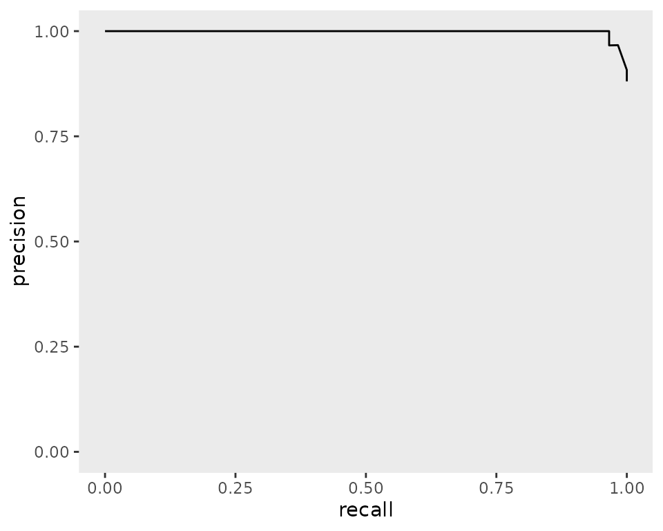
plotTopFeatsVI(results$fit, n_top_feats = 10)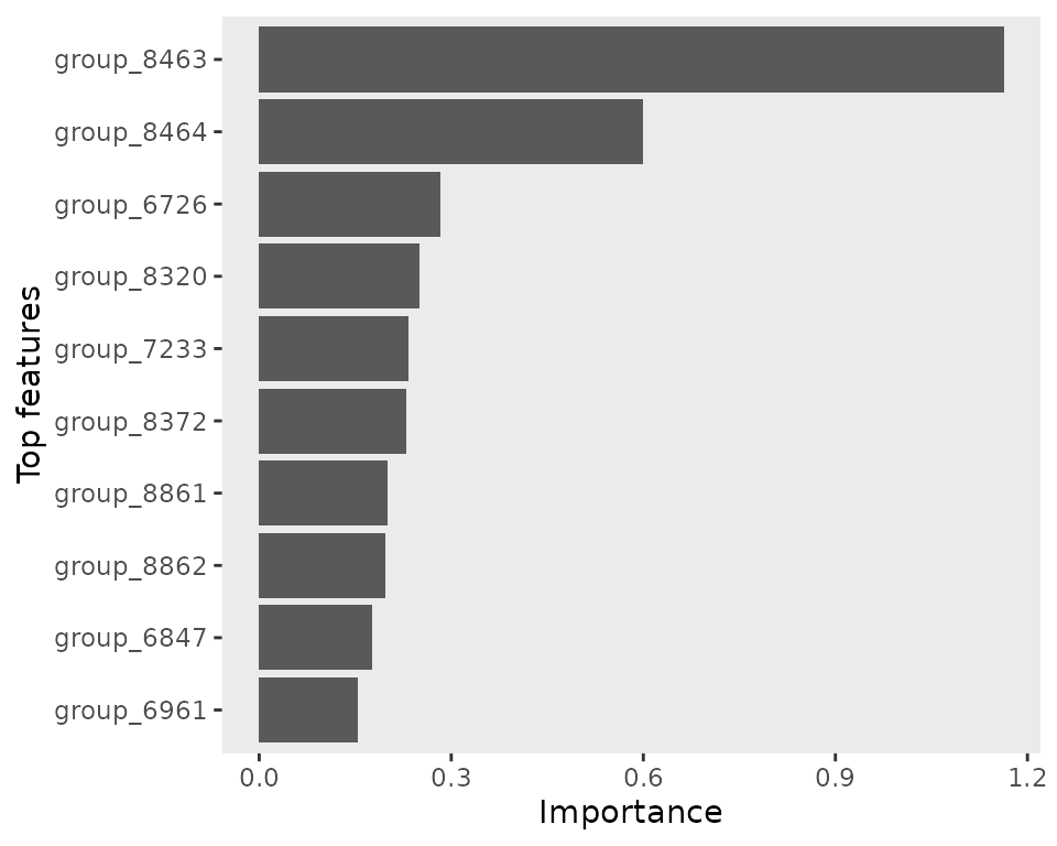
For a baseline comparison against random labels, fit a shuffled-label pipeline and compare:
shuffled <- runMLPipeline(
  ml_input_tibble = ml_tibble,
  model           = "LR",
  split           = c(1, 0),
  n_fold          = 2,
  shuffle_labels  = TRUE,
  return_pred     = TRUE
)

plotBaselineComparison(
  non_shuffled_label_results = results$performance_tibble,
  shuffled_label_results     = shuffled$performance_tibble
)
Iterative feature elimination
runIFE() retrains the model after iteratively removing
top-ranked features, helping identify the minimal predictive subset. It
runs the pipeline once per percentile in
percent_removal_vec
ife_results <- runIFE(
  ml_tibble,
  by_num              = TRUE,
  by_vi               = FALSE,
  percent_removal_vec = 10 * 1:9,
  mix_vec             = 0,
  return_feats        = TRUE,
  verbose             = FALSE
)

ife_results$ife_performance_tibble
ife_results$feats_removed
removeTopFeats() strips a given set of features from a
matrix tibble if you want to do this manually:
trimmed <- removeTopFeats(ml_tibble, head(top_features, 5))
ncol(ml_tibble) - ncol(trimmed)
#> [1] 5
Fisher’s exact tests (non-ML baseline)
runFishers() runs a Fisher’s exact test of feature
presence vs. phenotype for each feature, applies Benjamini–Hochberg
correction, and computes per-class frequencies.
fisher_results <- runFishers(
  matrix_path       = matrix_path,
  Q                 = 0.05,
  alternative       = "two.sided",
  susceptible_label = "Susceptible",
  resistant_label   = "Resistant"
)

head(fisher_results)
#> # A tibble: 6 × 8
#>   gene        p_value adj_p_value sig_after_bh alternative     Q
#>   <chr>         <dbl>       <dbl> <lgl>        <chr>       <dbl>
#> 1 group_8463 2.14e-32    1.49e-28 TRUE         two.sided    0.05
#> 2 group_8464 1.17e-26    4.06e-23 TRUE         two.sided    0.05
#> 3 group_6726 7.70e-23    1.78e-19 TRUE         two.sided    0.05
#> 4 group_6877 4.51e-21    7.84e-18 TRUE         two.sided    0.05
#> 5 group_7233 1.02e-20    1.42e-17 TRUE         two.sided    0.05
#> 6 group_6847 3.56e-20    3.67e-17 TRUE         two.sided    0.05
#> # ℹ 2 more variables: freq_susceptible_gene_pres <dbl>,
#> #   freq_resistant_gene_pres <dbl>
plotFishers(fisher_results, alpha = 0.05, label_top_n = 5)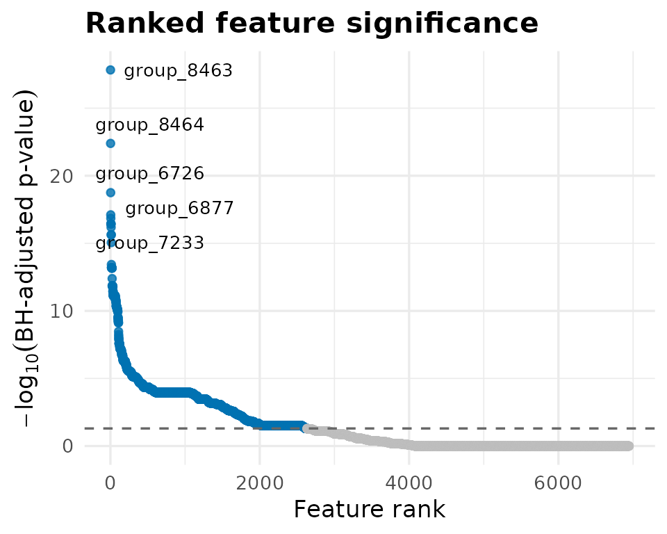
Training all models with runMLmodels
runMLmodels() trains a model on every matrix produced by
generateMLInputs() and writes performance TSVs into
out_path/ML_performance/, predictions into
ML_pred/, and top features into
ML_top_features/. Takes over an hour on Sfl with default
settings.
runMLmodels(
  path            = out_dir,
  stratify_by     = NULL,
  LOO             = FALSE,
  cross_test      = FALSE,
  threads         = max(1L, parallel::detectCores() - 1L),
  split           = c(1, 0),
  n_fold          = 5,
  verbose         = TRUE,
  return_pred     = TRUE,
  use_saved_split = TRUE
)
End-to-end: runModelingPipeline
For the full pipeline from a DuckDB to all outputs in one call:
runModelingPipeline(
  parquet_duckdb_path = fixture,
  threads             = max(1L, parallel::detectCores() - 1L),
  n_fold              = 5,
  split               = c(1, 0),
  min_n               = 25,
  prop_vi_top_feats   = c(0, 1),
  pca_threshold       = 0.99,
  verbose             = TRUE,
  use_saved_split     = TRUE
)
Session info
sessionInfo()
#> R version 4.6.1 (2026-06-24)
#> Platform: x86_64-pc-linux-gnu
#> Running under: Ubuntu 24.04.4 LTS
#>
#> Matrix products: default
#> BLAS:   /usr/lib/x86_64-linux-gnu/openblas-pthread/libblas.so.3
#> LAPACK: /usr/lib/x86_64-linux-gnu/openblas-pthread/libopenblasp-r0.3.26.so;  LAPACK version 3.12.0
#>
#> locale:
#>  [1] LC_CTYPE=C.UTF-8       LC_NUMERIC=C           LC_TIME=C.UTF-8
#>  [4] LC_COLLATE=C.UTF-8     LC_MONETARY=C.UTF-8    LC_MESSAGES=C.UTF-8
#>  [7] LC_PAPER=C.UTF-8       LC_NAME=C              LC_ADDRESS=C
#> [10] LC_TELEPHONE=C         LC_MEASUREMENT=C.UTF-8 LC_IDENTIFICATION=C
#>
#> time zone: UTC
#> tzcode source: system (glibc)
#>
#> attached base packages:
#> [1] stats     graphics  grDevices utils     datasets  methods   base
#>
#> other attached packages:
#> [1] amRml_0.99.0     BiocStyle_2.40.0
#>
#> loaded via a namespace (and not attached):
#>   [1] DBI_1.3.0           rlang_1.2.0         magrittr_2.0.5
#>   [4] tailor_0.1.0        furrr_0.4.0         otel_0.2.0
#>   [7] sgof_2.3.5          compiler_4.6.1      systemfonts_1.3.2
#>  [10] vctrs_0.7.3         stringr_1.6.0       tune_2.1.0
#>  [13] crayon_1.5.3        pkgconfig_2.0.3     shape_1.4.6.1
#>  [16] fastmap_1.2.0       labeling_0.4.3      utf8_1.2.6
#>  [19] rmarkdown_2.31      prodlim_2026.03.11  tzdb_0.5.0
#>  [22] ragg_1.5.2          purrr_1.2.2         bit_4.6.0
#>  [25] xfun_0.59           glmnet_5.0          cachem_1.1.0
#>  [28] jsonlite_2.0.0      recipes_1.3.3       vip_0.4.6
#>  [31] parallel_4.6.1      R6_2.6.1            bslib_0.11.0
#>  [34] stringi_1.8.7       rsample_1.3.2       RColorBrewer_1.1-3
#>  [37] parallelly_1.47.0   rpart_4.1.27        lubridate_1.9.5
#>  [40] jquerylib_0.1.4     Rcpp_1.1.1-1.1      bookdown_0.47
#>  [43] assertthat_0.2.1    dials_1.4.4         iterators_1.0.14
#>  [46] knitr_1.51          future.apply_1.20.2 poibin_1.6
#>  [49] readr_2.2.0         Matrix_1.7-5        splines_4.6.1
#>  [52] nnet_7.3-20         timechange_0.4.0    tidyselect_1.2.1
#>  [55] yaml_2.3.12         timeDate_4052.112   codetools_0.2-20
#>  [58] listenv_1.0.0       lattice_0.22-9      tibble_3.3.1
#>  [61] withr_3.0.3         S7_0.2.2            evaluate_1.0.5
#>  [64] future_1.70.0       desc_1.4.3          survival_3.8-6
#>  [67] pillar_1.11.1       BiocManager_1.30.27 foreach_1.5.2
#>  [70] generics_0.1.4      vroom_1.7.1         hms_1.1.4
#>  [73] ggplot2_4.0.3       scales_1.4.0        globals_0.19.1
#>  [76] class_7.3-23        glue_1.8.1          tools_4.6.1
#>  [79] data.table_1.18.4   gower_1.0.2         fs_2.1.0
#>  [82] grid_4.6.1          yardstick_1.4.0     tidyr_1.3.2
#>  [85] workflowsets_1.1.1  ipred_0.9-15        duckdb_1.5.4
#>  [88] cli_3.6.6           DiceDesign_1.10     textshaping_1.0.5
#>  [91] workflows_1.3.0     parsnip_1.6.0       lava_1.9.1
#>  [94] arrow_24.0.0        dplyr_1.2.1         gtable_0.3.6
#>  [97] sass_0.4.10         digest_0.6.39       ggrepel_0.9.8
#> [100] farver_2.1.2        htmltools_0.5.9     pkgdown_2.2.0
#> [103] lifecycle_1.0.5     hardhat_1.4.3       sparsevctrs_0.3.6
#> [106] bit64_4.8.2         MASS_7.3-65